A Metropolis algorithm in R - Part 2: Adaptive proposals

In the previous post, we built a Metropolis algorithm to estimate latitudinal temperature gradients, approximated by a generalised logistic function. Recall that the Metropolis algorithm works by proposing new parameter values and evaluating the joint posterior probability of the model with these values, against the posterior with the current values.

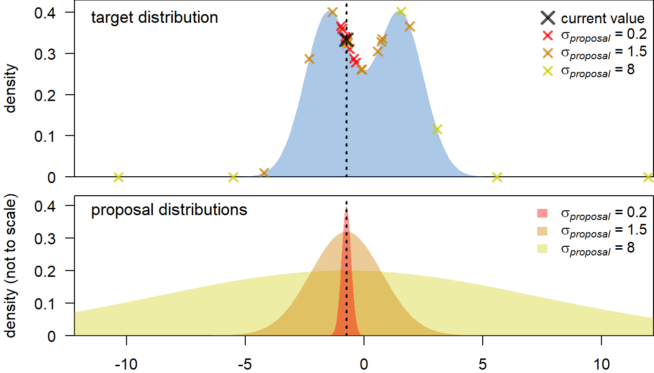
How do we chose a new value for a parameter? A common approach is to sample from a normal distribution, centred at the current value (i.e. the mean of the distribution is the current value). Choosing the standard deviation of the proposal distribution (\(\sigma_{proposal}\)) is more tricky. If \(\sigma_{proposal}\) is too high, we end up proposing a lot of values at the far tail ends of the target posterior distribution, which will usually be rejected (see below, yellow proposals). This leads to inefficient sampling and patchy coverage of the posterior distribution. Conversely, a very small \(\sigma_{proposal}\) leads to most new values being accepted, but the resulting Markov chain will move very slowly through the parameter space, leading to a low effective sample size (red proposals). Instead, some intermediate \(\sigma_{proposal}\) is desirable, at which the Markov chain moves quickly through the parameter space, without too many rejections (e.g., orange proposals).

It turns out that the Metropolis algorithm is usually most efficient when the acceptance rate of proposals is between $ 0.2$ and \(0.5\) (see Roberts and Rosenthal 2001). In practice, this could be achieved e.g. by monitoring the acceptance rate or the standard deviation of the target distribution (\(\sigma_{target}\)), and adjusting \(\sigma_{proposal}\) accordingly. Here, we will take the latter approach. For a four-dimensional Gaussian target distribution, the optimal \(\sigma_{proposal}\) should be around \(~2.4/sqrt(4) \times \sigma_{target}\) (Gelman et al. 1996), so we will adapt \(\sigma_{proposal}\) towards this target.

In order to allow for \(\sigma_{proposal}\) to quickly converge on the optimum, the square root of the weighted variance of the samples from the Markov chains from previous iterations is used as the \(\sigma_{proposal}\) for the next iteration. The weights decrease backwards in time, so that the recent values have more influence on the new value for \(\sigma_{proposal}\). The weighted variance is calculated with the following function, where x denotes a vector of samples from the Markov chain, weights a vector of weights (see below), and sum_weights records the sum of the weights vector:

weighted_var <- function(x, weights, sum_weights) {
  sum(weights*((x-sum(weights*x)/sum_weights)^2))/(sum_weights)
}

We can re-use most of the auxiliary functions of the standard Metropolis algorithm. Notably, the value of \(\sigma_{proposal}\) (propose_sd) will change during the adaptation.

MH_propose <- function(coeff, proposal_sd){
  rnorm(4,mean = coeff, sd= proposal_sd)
}

The specification of the weights and the adaption of \(\sigma_{proposal}\) is implemented in the updated MCMC loop. nAdapt specifies the number of iterations in which adaptations takes place. These iterations need to be discarded as burn-in to not bias the estimate of the posterior. adaptation_decay is a constant that influences the exponential decay of the weights for the weighted variance function, with larger values leading to slower decay.

Below is the full MCMC loop:

# Main MCMCM function
run_MCMC <- function(x, y, coeff_inits, sdy_init, nIter, proposal_sd_init = rep(5,4), 
                     nAdapt = 5000, adaptation_decay = 500){
  ### Initialisation
  coefficients = array(dim = c(nIter,4)) # set up array to store coefficients
  coefficients[1,] = coeff_inits # initialise coefficients
  sdy = rep(NA_real_,nIter) # set up vector to store sdy
  sdy[1] = sdy_init # intialise sdy
  A_sdy = 3 # parameter for the prior on the inverse gamma distribution of sdy
  B_sdy = 0.1 # parameter for the prior on the inverse gamma distribution of sdy
  n <- length(y)
  shape_sdy <- A_sdy+n/2 # shape parameter for the inverse gamma
  sd_it <- 1 # iteration index for the proposal standard deviation
  proposal_sd <- array(NA_real_,dim = c(nAdapt,4)) # array to store proposal SDs
  proposal_sd[1:3,] <- proposal_sd_init # proposal SDs before adaptation
  # pre-define exp. decaying weights for weighted variance
  allWeights <- exp((-(nAdapt-2)):0/adaptation_decay) 
  accept <- rep(NA,nIter) # vector to store the acceptance or rejection of proposals
  ### The MCMC loop
  for (i in 2:nIter){

   ## 1. Gibbs step to estimate sdy
    sdy[i] = sqrt(1/rgamma(
      1,shape_sdy,B_sdy+0.5*sum((y-gradient(x,coefficients[i-1,],0))^2)))

   ## 2. Metropolis-Hastings step to estimate the regression coefficients
    proposal = MH_propose(coefficients[i-1,],proposal_sd[sd_it,]) # new proposed values
    if(any(proposal[4] <= 0)) HR = 0 else {# Q and nu need to be >0
      # Hasting's ratio of the proposal
      HR = exp(logposterior(x = x, y = y, coeff = proposal, sdy = sdy[i]) -
                 logposterior(x = x, y = y, coeff = coefficients[i-1,], sdy = sdy[i]))}

    #if(gradient(65, proposal,0) >10) HR = 0
    # accept proposal with probability = min(HR,1)
    if (runif(1) < HR){
      accept[i] <- 1
      coefficients[i,] = proposal
      # if proposal is rejected, keep the values from the previous iteration
    }else{
      accept[i] <- 0
      coefficients[i,] = coefficients[i-1,]
    }
    # Adaptation of proposal SD
    if(i < nAdapt){ # stop adaptation after nAdapt iterations
    if(i>=3) {
    weights = allWeights[(nAdapt-i+2):nAdapt-1] # select weights for current iteration
    sum_weights = sum(weights) 
    weighted_var_coeff <- apply(coefficients[2:i,], 2, # calculate weighted variance
          function(f) weighted_var(
          f, weights = weights, sum_weights = sum_weights))

    for(v in 1:4) {if(weighted_var_coeff[v]==0)   { # if variance is zero, reduce sd
              proposal_sd[i+1,v] <- sqrt(proposal_sd[i,v]^2/5)
      } else  proposal_sd[i+1,v] <- 2.4/sqrt(4) * sqrt(weighted_var_coeff[v]) + 0.0001 
      # note that a small value is added to prevent that the adaptation gets stuck.
    }                   
                           
    }
    sd_it <- i+1 # index to access proposal_sd in the next iteration
    }
  } # end of the MCMC loop

  ###  Function output
  output = list(coeff = data.frame(A = coefficients[,1],
                           K = coefficients[,2],
                           M = coefficients[,3],
                           Q = coefficients[,4],
                           sdy = sdy),
                proposal_sd = data.frame(proposal_sd),
                accept = accept)
  # return output
    output
}

We re-use the data from the previous post, and set the initial standard deviation of the proposals to \(5\). This is probably too high, but we want to test whether the adaptation finds good values. We set the total number of iterations to \(100~000\), and use the first \(5000\) iterations as the adapation phase:

### Analysis
proposal_sd_init <- 5
nIter <- 100000
nAdapt <- 5000
m <- run_MCMC(x = sample_data$x, y = sample_data$y,
                                 coeff_inits = c(0,30,45,0.2), sdy_init = 4, 
                                 nIter = nIter, nAdapt = nAdapt, 
                                 adaptation_decay = nAdapt/10,
                                 proposal_sd_init = proposal_sd_init)

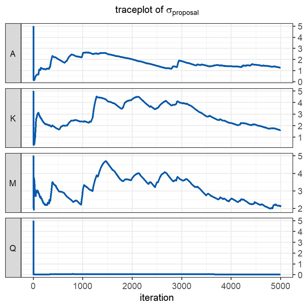
Looking at the traceplots, the MCMC runs well after an initial burn-in period, in which \(\sigma_{proposal}\) was adjusted. 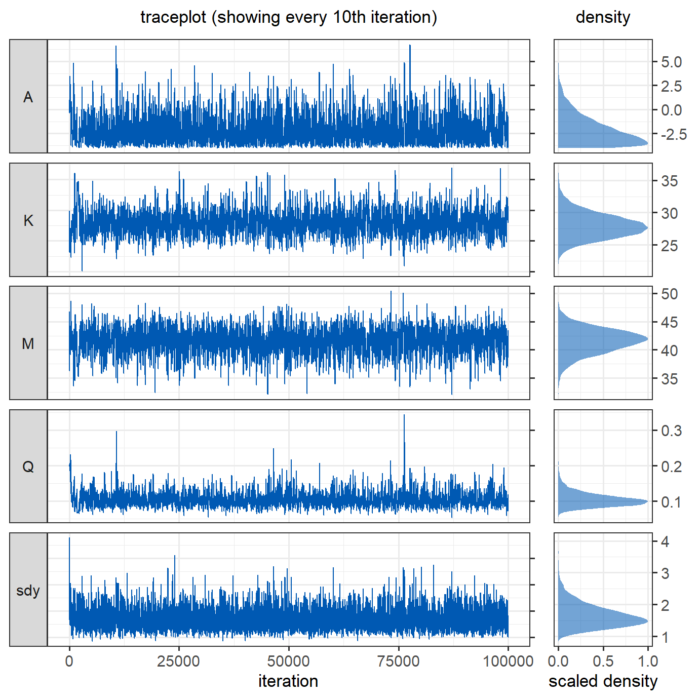The traceplot below shows how the standard deviations of the proposals were adapted during the first \(5000\) iterations. Despite a very bad initial guess for the \(\sigma_{proposal}\) of \(Q\), the adaptive algorithm managed to quickly find smaller, better values, resulting in reasonably good behaviour of the Markov chains of the parameters shown above. After the adaptation (at iteration \(5000\)), the most recent proposal values are used for the remainder of the iterations. The effective sample size after adaptation is \(3720\), which is \(52\%\) higher than the effective sample size obtained with the same number of iterations in the previous version of this model, where we tried to guess good values for \(\sigma_{proposal}\). Checking the acceptance rate shows that it is somewhat low even after the adaptation, at 0.16. In multi-dimensional models, a good acceptance rate would be around \(0.25\) (Gelman et al. 1997). To further improve this algorithm and achieve more efficient sampling at a higher acceptance rate, we could use multivariate proposals that account for the correlation of parameters (see e.g. Haario et al. 2001).

You can find the full R code to reproduce all analyses and figures on Github.