A Metropolis algorithm in R - Part 1: Implementation

The model presented herein uses modified code from https://khayatrayen.github.io/MCMC.html. I am currently developing a Metropolis-within-Gibbs algorithm for stratigraphic correlation of \(\delta\)¹³C records with Andrew R. Millard and Martin R. Smith at the Smith Lab at Durham University.

Markov chain Monte Carlo (MCMC) methods are widely used to obtain posterior probabilities for the unknown parameters of Bayesian models. The Metropolis algorithm builds a Markov chain for each parameter, which resembles the posterior distribution. This works by selecting arbitrary starting values for the parameters and calculating the resulting joint posterior probability. Then, new values for the parameters are randomly proposed, and the joint posterior probability is calculated with the new parameter values. If the posterior obtained with the new values is higher than that of the current values, the new values will be recorded and added to the Markov chains. Otherwise, the new value will be accepted with a probability equal to the ratio of the two posterior probabilities. If the proposed values result in a much lower posterior probability than the current values, the proposal will most likely be rejected. This process is repeated many times, and the resulting Markov chains converge on the posterior distributions of the parameters. The Metropolis algorithm requires symmetric proposal distributions and is a special case of the Metropolis-Hastings algorithm.

To illustrate the implementation of the Metropolis algorithm, we turn to climatology: Latitudinal temperature gradients from Earth history are difficult to reconstruct due to the sparse and geographically variable sampling of proxy data in most geological intervals. To reconstruct plausible temperature gradients from a fragmentary proxy record, classical solutions like LOESS or standard generalised additive models are not optimal, as earth scientists have additional information on past temperature gradients that those models do not incorporate. Instead, I propose the use of a generalised logistic function (a modified Richard’s curve) that can readily incorporate information in addition to the proxy data. For example, we can instruct the model to force temperature to continuously decrease from the tropics toward the poles.

To keep with the familiar notation in regression models, we set denote latitude as \(x\) and temperature as \(y\). Temperature is modelled as a function of latitude as:

\(\begin{aligned} \begin{equation} \begin{array}{l} y_i \sim N(\mu_i, \sigma), ~~\\ \mu_i = A~+max(K-A,0)/(e^{Q(x_i-M)}), ~~~~~ i = 1,...,n. \end{array} \end{equation} \end{aligned}\)

\(A\) is the lower asymptote, \(K\) is the upper asymptote, \(M\) is the inflection point, i.e. the steepest point of the curve, and \(Q\) controls the steepness of the curve. The difference \(K-A\) is constrained to be \(\ge 0\) to preclude inverse temperature gradients.

In R code, we turn this into a function named \(gradient\):

gradient <- function(x, coeff, sdy) { # sigma is labelled "sdy"
  A = coeff[1]
  K = coeff[2]
  M = coeff[3]
  Q = coeff[4]
  return(A + max(c(K-A,0))/((1+(exp(Q*(x-M))))) + rnorm(length(x),0,sdy))
}

As an example, let’s look at the modern, average latitudinal sea surface temperature gradient. We approximate it by setting \(A = -2.0\), \(K = 28\), \(M = 41\), and \(Q = 0.10\). The residual standard deviation \(\sigma\) is set to \(0\), resulting in a smooth curve without noise (lefthand plot). Note that we are using absolute latitudes, assuming a common latitudinal temperature gradient in both hemispheres. We also sample \(10\) points from this gradient, introducing some noise by setting \(\sigma = 2\) (righthand plot). In the following, we will use these \(10\) points to estimate a latitudinal gradient, using the gradient model specified above.

set.seed(10)
sample_lat <- runif(10,0,90)
sample_data <- data.frame(
  x = sample_lat, 
  y = gradient(x = sample_lat, coeff = c(-2.0, 28, 41, 0.1), sd = 2))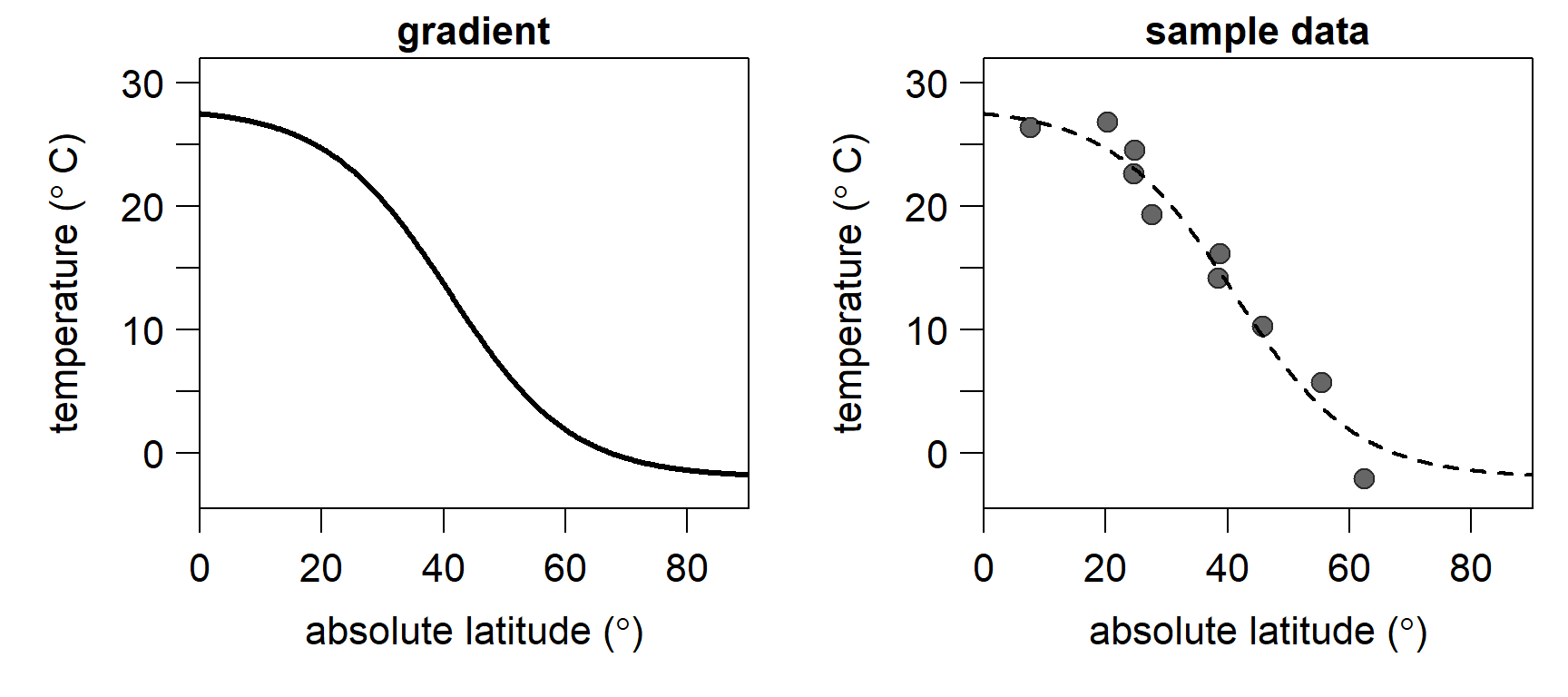

Before writing the main Markov chain Monte Carlo (MCMC) function, we pre-define a couple of supplementary functions that we use in every iteration of the Metropolis algorithm.

We start with the log-likelihood function, which translates to the joint probability of the data, given a specific set of model parameters:

loglik <- function(x, y,  coeff, sdy) {
  A = coeff[1]
  K = coeff[2]
  M = coeff[3]
  Q = coeff[4]
  pred = A + max(c(K-A,0))/((1+(exp(Q*(x-M)))))
  return(sum(dnorm(y, mean = pred, sd = sdy, log = TRUE)))
}

Next, we need a function to generate the log-priors, i.e. the joint prior probability of the set of model parameters. We specify the parameters of the prior distribution within the function for convenience. Uniform priors ranging from \(-4\) to \(40\) are put on \(A\) and \(K\), signifying that the temperature gradient cannot exceed this range. A normal prior with a mean of \(45\) and a standard deviation of \(10\) is placed on \(M\), implying that we expect the steepest temperature gradient in the mid-latitudes. We constrain \(Q\) to be \(>0\) by placing a log-normal prior on it:

logprior <- function(coeff) {
  return(sum(c(
    dunif(coeff[1], -4, 40, log = TRUE),
    dunif(coeff[2], -4, 40, log = TRUE),
    dnorm(coeff[3], 45, 10, log = TRUE),
    dlnorm(coeff[4], -2, 1, log = TRUE))))
}

The posterior is proportional to the likelihood \(\times\) prior. On the log scale, we can simply add them:

logposterior <- function(x, y, coeff, sdy){
  return (loglik(x, y, coeff, sdy) + logprior(coeff))
}

Finally, we define a function that proposes new values for the Metropolis-Hastings step. The magnitude of the proposal standard deviations (\(\sigma_{proposal}\)) is quite important, as low values will lead to the chain exploring the parameter space very slowly, and high values result in a low acceptance rate and an insufficient exploration of the parameter space. As appropriate \(\sigma_{proposal}\) are difficult to know a priori, adaptive steps are often used to find better values. For simplicity, we will use fixed \(\sigma_{proposal}\). Different \(\sigma_{proposal}\) can and usually should be used for different parameters.

MH_propose <- function(coeff, proposal_sd){
  return(rnorm(4,mean = coeff, sd= c(.5,.5,.5,0.01)))
}

With all the prerequisites in place, we can build the MCMC function. The model will update \(\sigma\) with a Gibbs step, and update the other coefficients with a Metropolis-Hastings step:

run_MCMC <- function(x, y, coeff_inits, sdy_init, nIter){
  ### Initialisation
  coefficients = array(dim = c(nIter,4)) # set up array to store coefficients
  coefficients[1,] = coeff_inits # initialise coefficients
  sdy = rep(NA_real_,nIter) # set up vector to store sdy
  sdy[1] = sdy_init # intialise sdy
  A_sdy = 3 # parameter for the prior on the inverse gamma distribution of sdy
  B_sdy = 0.1 # parameter for the prior on the inverse gamma distribution of sdy
  n <- length(y)
  shape_sdy <- A_sdy+n/2 # shape parameter for the inverse gamma
  
  ### The MCMC loop
  for (i in 2:nIter){ 
    
    ## 1. Gibbs step to estimate sdy
    sdy[i] = sqrt(1/rgamma(
      1,shape_sdy,B_sdy+0.5*sum((y-gradient(x,coefficients[i-1,],0))^2)))
    
    ## 2. Metropolis-Hastings step to estimate the regression coefficients
    proposal = MH_propose(coefficients[i-1,]) # new proposed values
    if(any(proposal[4] <= 0)) HR = 0 else # Q needs to be >0
    # Hastings ratio of the proposal
    HR = exp(logposterior(x = x, y = y, coeff = proposal, sdy = sdy[i]) -
             logposterior(x = x, y = y, coeff = coefficients[i-1,], sdy = sdy[i]))
    # accept proposal with probability = min(HR,1)
    if (runif(1) < HR){ 
      coefficients[i,] = proposal
    # if proposal is rejected, keep the values from the previous iteration
    }else{
      coefficients[i,] = coefficients[i-1,]
    }
  } # end of the MCMC loop
  
  ###  Function output
  output = data.frame(A = coefficients[,1],
                      K = coefficients[,2],
                      M = coefficients[,3],
                      Q = coefficients[,4],
                      sdy = sdy)
  return(output)
}

To run the model, we need to provide starting values for the unknown parameters. We let it run for \(100,000\) iterations:

nIter <- 100000
m <- run_MCMC(x = sample_data$x, y = sample_data$y, 
              coeff_inits = c(0,30,45,0.2), sdy_init = 4, nIter = nIter)

To assess the model output, we produce trace plots and density plots of the posterior estimates of the parameters. For the trace plot, only every \(10^{th}\) iteration is shown to improve readability. The black lines in the density plot denote the parameters of the original sea surface temperature gradient. 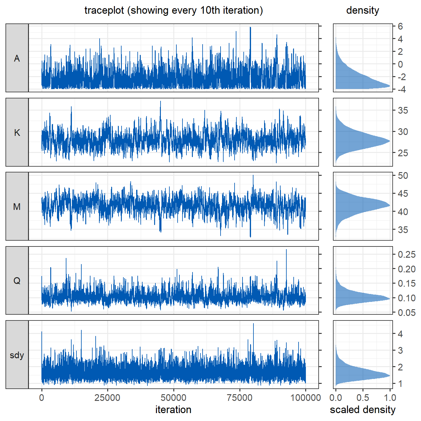The parameters have converged reasonably well.

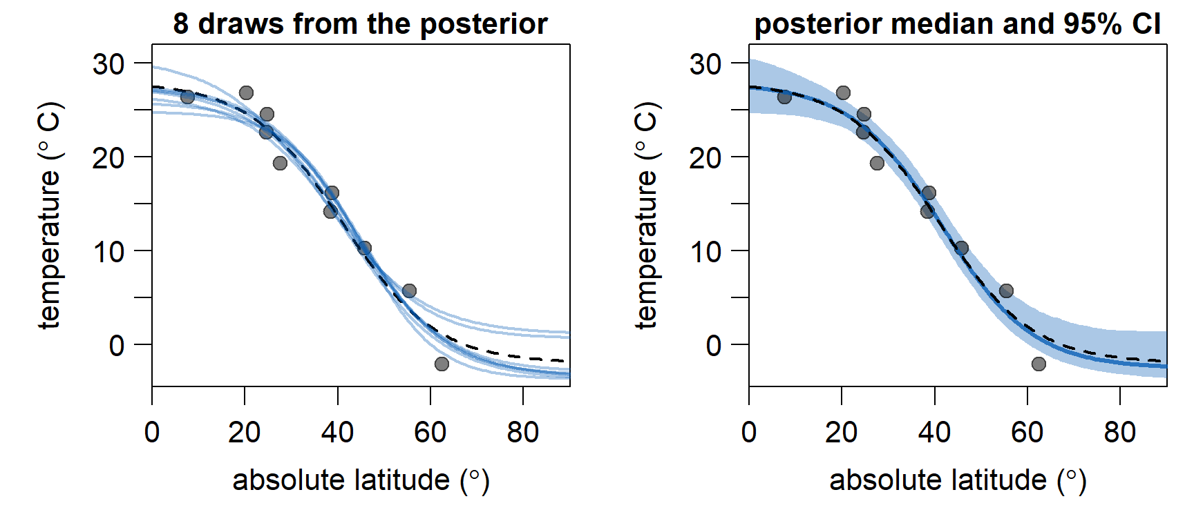
Below, we discard the first \(10,000\) iterations as burn-in and plot \(8\) gradients, using different samples from the posterior (blue lines, lefthand plot). As expected, they fit nicely to the \(10\) sampled data points (grey dots). They are also quite similar to the original gradient (black, dashed line). To the right, the estimated temperature gradient using the median of the parameters from the posterior (blue line), and \(95\%\) credible intervals (blue shading), are shown. Between \(10^\circ\) and \(50^\circ\), where we have sufficient samples, the estimated gradient very closely resembles the original gradient. The constraints imposed by the priors ensure that the estimated sea surface temperature gradients stays in a realistic range (\(>-4^\circ C\)), even at latitudes \(> 63^\circ\) where we have no data.

In conclusion, the model seems to be doing a good job in estimating a sensible temperature gradient from sparse samples. In the second part of this series, we will implement adaption of \(\sigma_{proposal}\), which means we won’t have to guess good values for \(\sigma_{proposal}\). This should speed up convergence, meaning we will need less iterations of the MCMC algorithm to obtain reliable posterior estimates.

You can find the full R code to reproduce all analyses and figures on Github.